=== The asymptotic expansion in the case of a single non-degenerate saddle point ===
=== The asymptotic expansion in the case of a single non-degenerate saddle point ===
Assume
Assume
# <math>f(z)</math> and <math>S(z)</math> are [[Holomorphic function|holomorphic]] functions in an [[Open set|open]], [[Bounded set (topological vector space)|bounded]], and [[Simply connected space|simply connected]] set <math>\Omega_x\subset \mathbb{C}^n</math> such that the set <math>I_x = \Omega_x\cap\mathbb{R}^n</math> is [[Connected space|connected]];
# {{math| ''f'' (''z'')}} and {{math|''S''(''z'')}} are [[Holomorphic function|holomorphic]] functions in an [[Open set|open]], [[Bounded set (topological vector space)|bounded]], and [[Simply connected space|simply connected]] set {{math|Ω''<sub>x</sub>'' ⊂ '''C'''<sup>''n''</sup>}} such that the {{math|''I<sub>x</sub>'' {{=}} Ω''<sub>x</sub>'' ∩ '''R'''<sup>''n''</sup>}} is [[Connected space|connected]];
# <math>\Re[S(z)]</math> has a single maximum: <math>\max\limits_{z\in I_x} \Re[S(z)] = \Re[S(x^0)]</math> for exactly one point <math>x^0 \in I_x </math>;
# <math>\Re(S(z))</math> has a single maximum: <math>\max\limits_{z \in I_x} \Re(S(z)) = \Re(S(x^0))</math> for exactly one point {{math|''x''<sup>0</sup> ∈ ''I<sub>x</sub>''}};
# <math>x^0</math> is a non-degenerate saddle point (i.e., <math>\nabla S(x^0) = 0</math> and <math>\det S''_{xx}(x^0) \neq 0</math>).
# {{math|''x''<sup>0</sup>}} is a non-degenerate saddle point (i.e., <math>\nabla S(x^0) = 0</math> and <math>\det S''_{xx}(x^0) \neq 0</math>).
where {{math|''μ<sub>j</sub>''}} are eigenvalues of the [[Hessian matrix|Hessian]] <math>S''_{xx}(x^0)</math> and <math>(-\mu_j)^{-\frac{1}{2}}</math> are defined with arguments
where <math>\mu_j</math> are eigenvalues of the [[Hessian matrix|Hessian]] <math>S''_{xx}(x^0)</math> and <math>(-\mu_j)^{-1/2}</math> are defined with arguments
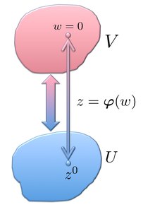
[[File:Illustration To Derivation Of Asymptotic For Saddle Point Integration.pdf|thumb|center|An illustration to the derivation of equation (8)]]
[[File:Illustration To Derivation Of Asymptotic For Saddle Point Integration.pdf|thumb|center|An illustration to the derivation of equation (8)]]
First, we deform the contour <math>I_x</math> into a new contour <math>I'_x \subset \Omega_x</math> passing through the saddle point <math>x^0</math> and sharing the boundary with <math>I_x</math>. This deformation does not change the value of the integral <math>I(\lambda)</math>. We employ the [[Method_of_steepest_descent#Complex_Morse_Lemma|Complex Morse Lemma]] to change the variables of integration. According to the lemma, the function <math>\boldsymbol{\varphi}(w)</math> maps a neighborhood <math>U \subset \Omega_x</math> (<math>x^0 \in U</math>) onto a neighborhood <math>\Omega_w</math> containing the origin. The integral <math>I(\lambda)</math> can be split into two: <math>I(\lambda) = I_0(\lambda) + I_1(\lambda)</math>, where <math>I_0(\lambda)</math> is the integral over <math>U\cap I'_x</math>, while <math>I_1(\lambda)</math> is over <math>I'_x \setminus (U\cap I'_x)</math> (i.e., the remaining part of the contour <math>I'_x</math>). Since the latter region does not contain the saddle point <math>x^0</math>, the value of <math>I_1(\lambda)</math> is exponentially smaller than <math>I_0(\lambda)</math> as <math>\lambda\to+\infty</math>;<ref> This conclusion follows from a comparison between the final asymptotic for <math>I_0(\lambda)</math>, given by equation (8), and [[Method_of_steepest_descent#A_simple_estimate_.5B1.5D|a simple estimate]] for the discarded integral <math>I_1(\lambda)</math>.</ref> thus, <math>I_1(\lambda)</math> is ignored. Introducing the contour <math>I_w</math> such that <math>U\cap I'_x = \boldsymbol{\varphi}(I_w)</math>, we have
First, we deform the contour {{math|''I<sub>x</sub>''}} into a new contour <math>I'_x \subset \Omega_x</math> passing through the saddle point {{math|''x''<sup>0</sup>}} and sharing the boundary with {{math|''I<sub>x</sub>''}}. This deformation does not change the value of the integral {{math|''I''(''λ'')}}. We employ the [[Method_of_steepest_descent#Complex_Morse_Lemma|Complex Morse Lemma]] to change the variables of integration. According to the lemma, the function {{math|'''''φ'''''(''w'')}} maps a neighborhood {{math|''x''<sup>0</sup> ∈ ''U'' ⊂ Ω''<sub>x</sub>''}} onto a neighborhood {{math|Ω''<sub>w</sub>''}} containing the origin. The integral {{math|''I''(''λ'')}} can be split into two: {{math|''I''(''λ'') {{=}} ''I''<sub>0</sub>(''λ'') + ''I''<sub>1</sub>(''λ'')}}, where {{math|''I''<sub>0</sub>(''λ'')}} is the integral over <math>U\cap I'_x</math>, while {{math|''I''<sub>1</sub>(''λ'')}} is over <math>I'_x \setminus (U\cap I'_x)</math> (i.e., the remaining part of the contour <math>I'_x</math>). Since the latter region does not contain the saddle point {{math|''x''<sup>0</sup>}}, the value of {{math|''I''<sub>1</sub>(''λ'')}} is exponentially smaller than {{math|''I''<sub>0</sub>(''λ'')}} as {{math|''λ'' → ∞}};<ref> This conclusion follows from a comparison between the final asymptotic for {{math|''I''<sub>0</sub>(''λ'')}}, given by equation (8), and [[Method_of_steepest_descent#A_simple_estimate_.5B1.5D|a simple estimate]] for the discarded integral {{math|''I''<sub>1</sub>(''λ'')}}.</ref> thus, {{math|''I''<sub>1</sub>(''λ'')}} is ignored. Introducing the contour {{math|''I<sub>w</sub>''}} such that <math>U\cap I'_x = \boldsymbol{\varphi}(I_w)</math>, we have
Recalling that <math>x^0 = \boldsymbol{\varphi}(0)</math> as well as <math>\det \boldsymbol{\varphi}_w'(0) = 1</math>, we expand the pre-exponential function into a Taylor series and keep just the leading zero-order term
Recalling that {{math|''x''<sup>0</sup> {{=}} '''''φ'''''(0)}} as well as <math>\det \boldsymbol{\varphi}_w'(0) = 1</math>, we expand the pre-exponential function into a Taylor series and keep just the leading zero-order term
Here, we have substituted the integration region <math>I_w</math> by <math>\mathbb{R}^n</math> because both contain the origin, which is a saddle point, hence they are equal up to an exponentially small term.<ref>This is justified by comparing the integral asymptotic over <math>\mathbb{R}^n</math> [see equation (8)] with [[Method_of_steepest_descent#A_simple_estimate_.5B1.5D|a simple estimate]] for the altered part.</ref> The integrals in the r.h.s. of equation (11) can be expressed as
Here, we have substituted the integration region {{math|''I<sub>w</sub>''}} by {{math|'''R'''<sup>''n''</sup>}} because both contain the origin, which is a saddle point, hence they are equal up to an exponentially small term.<ref>This is justified by comparing the integral asymptotic over {{math|'''R'''<sup>''n''</sup>}} [see equation (8)] with [[Method_of_steepest_descent#A_simple_estimate_.5B1.5D|a simple estimate]] for the altered part.</ref> The integrals in the r.h.s. of equation (11) can be expressed as
From this representation, we conclude that condition (9) must be satisfied in order for the r.h.s. and l.h.s. of equation (12) to coincide. According to assumption 2, <math>\Re[ S_{xx}''(x^0) ]</math> is a [[Definite bilinear form|negatively defined quadratic form]] (viz., <math>\Re(\mu_j)<0</math>) implying the existence of the integral <math>\mathcal{I}_j</math>, which is readily calculated
From this representation, we conclude that condition (9) must be satisfied in order for the r.h.s. and l.h.s. of equation (12) to coincide. According to assumption 2, <math>\Re \left( S_{xx}''(x^0) \right)</math> is a [[Definite bilinear form|negatively defined quadratic form]] (viz., <math>\Re(\mu_j)<0</math>) implying the existence of the integral <math>\mathcal{I}_j</math>, which is readily calculated
* If <math> S(x) </math> is real valued for real ''x'' and <math> x^0 \in \mathbb{R}^n</math> (aka, the '''multidimensional Laplace method'''), then <math> {\rm Ind} (-S_{xx}''(x^0)) = 0 </math>.<ref>See equation (4.4.9) on page 125 in {{harvtxt|Fedoryuk|1987}}</ref>
* If {{math|''S''(''x'')}} is real valued for real {{mvar|x}} and {{math|''x''<sup>0</sup>}} in {{math|'''R'''<sup>''n''</sup>}} (aka, the '''multidimensional Laplace method'''), then<ref>See equation (4.4.9) on page 125 in {{harvtxt|Fedoryuk|1987}}</ref>
* If {{math|''S''(''x'')}} is purely imaginary for real {{mvar|x}} (i.e., <math>\Re(S(x)) = 0</math> for all {{mvar|x}} in {{math|'''R'''<sup>''n''</sup>}}) and {{math|''x''<sup>0</sup>}} in {{math|'''R'''<sup>''n''</sup>}} (aka, the '''multidimensional stationary phase method'''),<ref>Rigorously speaking, this case cannot be inferred from equation (8) because [[Method_of_steepest_descent#The_asymptotic_expansion_in_the_case_of_a_single_non-degenerate_saddle_point|the second assumption]], utilized in the derivation, is violated. To include the discussed case of a purely imaginary phase function, condition (9) should be replaced by <math> \left | \arg\sqrt{-\mu_j} \right | \leqslant \tfrac{\pi}{4}.</math></ref> then<ref>See equation (2.2.6') on page 186 in {{harvtxt|Fedoryuk|1987}}</ref>
:where <math>\text{sign }S_{xx}''(x_0)</math> denotes [[Sylvester's_law_of_inertia#Statement_of_the_theorem|the signature of matrix]] <math>S_{xx}''(x_0)</math>, which equals to the number of negative eigenvalues minus the number of positive ones. It is noteworthy that in applications of the stationary phase method to the multidimensional WKB approximation in quantum mechanics (as well as in optics), {{math|Ind}} is related to the [[Maslov index]] see, e.g., {{harvtxt|Chaichian|Demichev|2001}} and {{harvtxt|Schulman|2005}}.
* If <math> S(x) </math> is purely imaginary for real ''x'' (i.e., <math>\Re[S(x)] = 0,\,\forall x \in \mathbb{R}^n</math>) and <math> x^0 \in \mathbb{R}^n</math> (aka, the '''multidimensional stationary phase method'''),<ref>Rigorously speaking, this case cannot be inferred from equation (8) because [[Method_of_steepest_descent#The_asymptotic_expansion_in_the_case_of_a_single_non-degenerate_saddle_point|the second assumption]], utilized in the derivation, is violated. To include the discussed case of a purely imaginary phase function, condition (9) should be replaced by <math> | \arg\sqrt{-\mu_j}| \leqslant \pi/4</math>.</ref> then<ref>See equation (2.2.6') on page 186 in {{harvtxt|Fedoryuk|1987}}</ref> <math>
</math> where <math>{\rmsign}S_{xx}''(x_0)</math> denotes [[Sylvester's_law_of_inertia#Statement_of_the_theorem|the signature of matrix]] <math>S_{xx}''(x_0)</math>, which equals to the number of negative eigenvalues minus the number of positive ones. It is noteworthy that in applications of the stationary phase method to the multidimensional WKB approximation in quantum mechanics (as well as in optics), <math>{\rm Ind}</math> is related to the [[Maslov index]] see, e.g., {{harvtxt|Chaichian|Demichev|2001}} and {{harvtxt|Schulman|2005}}.
== The case of multiple non-degenerate saddle points ==
== The case of multiple non-degenerate saddle points ==
In mathematics, the method of steepest descent or stationary phase method or saddle-point method is an extension of Laplace's method for approximating an integral, where one deforms a contour integral in the complex plane to pass near a stationary point (saddle point), in roughly the direction of steepest descent or stationary phase. The saddle-point approximation is used with integrals in the complex plane, whereas Laplace’s method is used with real integrals.
The integral to be estimated is often of the form
where C is a contour and λ is large. One version of the method of steepest descent deforms the contour of integration
so that it passes through a zero of the derivative g′(z) in such a way that on the contour g is (approximately) real and has a maximum at the zero.
The method of steepest descent was first published by Debye (1909), who used it to estimate Bessel functions and pointed out that it occurred in the unpublished note Riemann (1863) about hypergeometric functions. The contour of steepest descent has a minimax property, see Fedoryuk (2001) harvtxt error: no target: CITEREFFedoryuk2001 (help). Siegel (1932) described some other unpublished notes of Riemann, where he used this method to derive the Riemann-Siegel formula.
is a vector function, then its Jacobian matrix is defined as
A non-degenerate saddle point, , of a holomorphic function is a point where the function reaches an extremum (i.e., ) and has a non-vanishing determinant of the Hessian (i.e., ).
The following is the main tool for constructing the asymptotics of integrals in the case of a non-degenerate saddle point:
Complex Morse Lemma
The Morse lemma for real-valued functions generalizes as follows[2] for holomorphic functions: near a non-degenerate saddle point of a holomorphic function , there exist coordinates in terms of which is quadratic. Let S be a holomorphic function with domain , and let be a non-degenerate saddle point of S, that is, and . Then there exist neighborhoods of and of , and a bijective holomorphic function with such that
at all points . Here, the are the eigenvalues of the matrix .
An illustration of Complex Morse Lemma
Proof of Complex Morse Lemma
The following proof is a straightforward generalization of the proof of the real Morse Lemma, which can be found in.[3] We begin by demonstrating
Auxiliary Statement. Let be holomorphic in a neighborhood of the origin and . Then in some neighborhood, there exist functions such that , where each is holomorphic and .
Proof of Auxiliary Statement
From the identity
we conclude that
and
Without loss of generality, we translate the origin to , such that and . Using the Auxiliary Statement, we have
Since the origin is a saddle point,
we can also apply the Auxiliary Statement to the functions and obtain
(1)
Recall that an arbitrary matrix A can be represented as a sum of symmetric and anti-symmetric matrices,
The contraction of any symmetric matrix B with an arbitrary matrix A is
(2)
i.e., the anti-symmetric component of A does not contribute because
Thus, in equation (1) can be assumed to be symmetric with respect to the interchange of the indices i and j. Note that
hence, because the origin is a non-degenerate saddle point.
Let us show by induction that there are local coordinates , such that
(3)
First, assume that there exist local coordinates , , , such that
(4)
where is symmetric due to equation (2). By a linear change of the variables , we can assure that . From the chain rule, we have
Therefore:
whence,
The matrix can be recast in the Jordan normal form: , were L gives the desired non-singular linear transformation and the diagonal of J contains non-zero eigenvalues of . If then, due to continuity of , it must be also non-vanishing in some neighborhood of the origin. Having introduced , we write
Motivated by the last expression, we introduce new coordinates , ,
The change of the variables is locally invertible since the corresponding Jacobian is non-zero,
Therefore,
(5)
Comparing equations (4) and (5), we conclude that equation (3) is verified. Denoting the eigenvalues of by , equation (3) can be rewritten as
(6)
Therefore,
(7)
From equation (6), it follows that . The Jordan normal form of reads , where is an upper diagonal matrix containing the eigenvalues and ; hence, . We obtain from equation (7)
If , then interchanging two variables assures that .
The asymptotic expansion in the case of a single non-degenerate saddle point
has a single maximum: for exactly one point x0 ∈ Ix;
x0 is a non-degenerate saddle point (i.e., and ).
Then, the following asymptotic holds
(8)
where μj are eigenvalues of the Hessian and are defined with arguments
(9)
This statement is a special case of more general results presented in.[4]
Derivation of equation (8)
An illustration to the derivation of equation (8)
First, we deform the contour Ix into a new contour passing through the saddle point x0 and sharing the boundary with Ix. This deformation does not change the value of the integral I(λ). We employ the Complex Morse Lemma to change the variables of integration. According to the lemma, the function φ(w) maps a neighborhood x0 ∈ U ⊂ Ωx onto a neighborhood Ωw containing the origin. The integral I(λ) can be split into two: I(λ) = I0(λ) + I1(λ), where I0(λ) is the integral over , while I1(λ) is over (i.e., the remaining part of the contour ). Since the latter region does not contain the saddle point x0, the value of I1(λ) is exponentially smaller than I0(λ) as λ → ∞;[5] thus, I1(λ) is ignored. Introducing the contour Iw such that , we have
(10)
Recalling that x0 = φ(0) as well as , we expand the pre-exponential function into a Taylor series and keep just the leading zero-order term
(11)
Here, we have substituted the integration region Iw by Rn because both contain the origin, which is a saddle point, hence they are equal up to an exponentially small term.[6] The integrals in the r.h.s. of equation (11) can be expressed as
(12)
From this representation, we conclude that condition (9) must be satisfied in order for the r.h.s. and l.h.s. of equation (12) to coincide. According to assumption 2, is a negatively defined quadratic form (viz., ) implying the existence of the integral , which is readily calculated
Equation (8) can also be written as
(13)
where the branch of
is selected as follows
Consider important special cases:
If S(x) is real valued for real x and x0 in Rn (aka, the multidimensional Laplace method), then[7]
If S(x) is purely imaginary for real x (i.e., for all x in Rn) and x0 in Rn (aka, the multidimensional stationary phase method),[8] then[9]
where denotes the signature of matrix, which equals to the number of negative eigenvalues minus the number of positive ones. It is noteworthy that in applications of the stationary phase method to the multidimensional WKB approximation in quantum mechanics (as well as in optics), Ind is related to the Maslov index see, e.g., Chaichian & Demichev (2001) and Schulman (2005).
The case of multiple non-degenerate saddle points
If the function has multiple isolated non-degenerate saddle points (i.e., where is an open cover of ), calculation of the integral asymptotic is reduced to the case of a singe saddle point by employing the partition of unity.
The partition of unity allows us to construct a set of continuous functions such that and each function vanishes outside . Whence,
where equation (13) was utilized at the last stage, and the pre-exponential function at least must be continuous.
The other cases
When and , the point is called a degenerate saddle point of a function .
Calculating the asymptotic of , when , is continuous, and has a degenerate saddle point, is a very rich problem, whose solution heavily relies on the catastrophe theory. Here, the catastrophe theory replaces the Morse lemma, valid only in the non-degenerate case, to transform the function into one of the multitude of canonical representations. For further details see, e.g., Poston & Stewart (1978) and Fedoryuk (1987).
Integrals with degenerate saddle points naturally appear in many applications including optical caustics and the multidimensional WKB approximation in quantum mechanics.
The other cases such as, e.g., and/or are discontinuous or when an extremum of lies at the integration region's boundary, require special care (see, e.g., Fedoryuk (1987) and Wong (1989)).
Extensions and generalizations
An extension of the steepest descent method is the so-called nonlinear stationary phase/steepest descent method. Here, instead of integrals, one needs to evaluate asymptotically solutions of Riemann–Hilbert factorization problems.
Given a contour C in the complex sphere, a function f defined on that contour and a special point, say infinity, one seeks a function M holomorphic away from the contour C, with prescribed jump across C, and with a given normalization at infinity. If f and hence M are matrices rather than scalars this is a problem that in general does not admit an explicit solution.
An asymptotic evaluation is then possible along the lines of the linear stationary phase/steepest descent method. The idea is to reduce asymptotically the solution of the given Riemann–Hilbert problem to that of a simpler, explicitly solvable, Riemann–Hilbert problem. Cauchy's theorem is used to justify deformations of the jump contour.
The nonlinear stationary phase was introduced by Deift and Zhou in 1993, based on earlier work of the Russian mathematician Alexander Its. A (properly speaking) nonlinear steepest descent method was introduced by Kamvissis, K. McLaughlin and P. Miller in 2003, based on previous work of Lax, Levermore, Deift, Venakides and Zhou. As in the linear case, steepest descent contours solve a min-max problem.
^ This conclusion follows from a comparison between the final asymptotic for I0(λ), given by equation (8), and a simple estimate for the discarded integral I1(λ).
^This is justified by comparing the integral asymptotic over Rn [see equation (8)] with a simple estimate for the altered part.
^Rigorously speaking, this case cannot be inferred from equation (8) because the second assumption, utilized in the derivation, is violated. To include the discussed case of a purely imaginary phase function, condition (9) should be replaced by
Chaichian, M.; Demichev, A. (2001), Path Integrals in Physics Volume 1: Stochastic Process and Quantum Mechanics, Taylor & Francis, p. 174, ISBN075030801X
Debye, P. (1909), "Näherungsformeln für die Zylinderfunktionen für große Werte des Arguments und unbeschränkt veränderliche Werte des Index", Mathematische Annalen, 67 (4): 535–558, doi:10.1007/BF01450097 English translation in Debye, Peter J. W. (1954), The collected papers of Peter J. W. Debye, Interscience Publishers, Inc., New York, ISBN978-0-918024-58-9, MR0063975
Deift, P.; Zhou, X. (1993), "A steepest descent method for oscillatory Riemann-Hilbert problems. Asymptotics for the MKdV equation", Ann. Of Math., vol. 137, no. 2, The Annals of Mathematics, Vol. 137, No. 2, pp. 295–368, doi:10.2307/2946540, JSTOR2946540.
Fedoryuk, M. V. (1987), Asymptotic: Integrals and Series, Nauka, Moscow [in Russian].
Kamvissis, S.; McLaughlin, K. T.-R.; Miller, P. (2003), "Semiclassical Soliton Ensembles for the Focusing Nonlinear Schrödinger Equation", Annals of Mathematics Studies, vol. 154, Princeton University Press.
Riemann, B. (1863), Sullo svolgimento del quoziente di due serie ipergeometriche in frazione continua infinita (Unpublished note, reproduced in Riemann's collected papers.)
Siegel, C. L. (1932), "Über Riemanns Nachlaß zur analytischen Zahlentheorie", Quellen Studien zur Geschichte der Math. Astron. und Phys. Abt. B: Studien 2: 45–80 Reprinted in Gesammelte Abhandlungen, Vol. 1. Berlin: Springer-Verlag, 1966.
Poston, T.; Stewart, I. (1978), Catastrophe Theory and Its Applications, Pitman.
Schulman, L. S. (2005), "Ch. 17: The Phase of the Semiclassical Amplitude", Techniques and Applications of Path Integration, Dover, ISBN0486445283
Wong, R. (1989), Asymptotic approximations of integrals, Academic Press.