Multinomial logistic regression

"Multinomial regression" redirects here. For the related Probit procedure, see Multinomial probit.

In statistics, multinomial logistic regression is a classification method that generalizes logistic regression to multiclass problems, i.e. with more than two possible discrete outcomes. That is, it is a model that is used to predict the probabilities of the different possible outcomes of a categorically distributed dependent variable, given a set of independent variables (which may be real-valued, binary-valued, categorical-valued, etc.).

Multinomial logistic regression is known by a variety of other names, including polytomous LR, multiclass LR, softmax regression, multinomial logit, maximum entropy (MaxEnt) classifier, conditional maximum entropy model.

Introduction

Multinomial logistic regression is used when the dependent variable in question is nominal (equivalently categorical, meaning that it falls into any one of a set of categories which cannot be ordered in any meaningful way) and for which there are more than two categories. Some examples would be:

• Which major will a college student choose, given their grades, stated likes and dislikes, etc.?
• Which blood type does a person have, given the results of various diagnostic tests?
• In a hands-free mobile phone dialing application, which person's name was spoken, given various properties of the speech signal?
• Which candidate will a person vote for, given particular demographic characteristics?
• Which country will a firm locate an office in, given the characteristics of the firm and of the various candidate countries?

These are all statistical classification problems. They all have in common a dependent variable to be predicted that comes from one of a limited set of items which cannot be meaningfully ordered, as well as a set of independent variables (also known as features, explanators, etc.), which are used to predict the dependent variable. Multinomial logit regression is a particular solution to the classification problem that assumes that a linear combination of the observed features and some problem-specific parameters can be used to determine the probability of each particular outcome of the dependent variable. The best values of the parameters for a given problem are usually determined from some training data (e.g. some people for whom both the diagnostic test results and blood types are known, or some examples of known words being spoken).

Assumptions

The multinomial logit model assumes that data are case specific; that is, each independent variable has a single value for each case. The multinomial logit model also assumes that the dependent variable cannot be perfectly predicted from the independent variables for any case. As with other types of regression, there is no need for the independent variables to be statistically independent from each other (unlike, for example, in a naive Bayes classifier); however, collinearity is assumed to be relatively low, as it becomes difficult to differentiate between the impact of several variables if this is not the case.

If the multinomial logit is used to model choices, it relies on the assumption of independence of irrelevant alternatives (IIA), which is not always desirable. This assumption states that the odds of preferring one class over another do not depend on the presence or absence of other "irrelevant" alternatives. For example, the relative probabilities of taking a car or bus to work do not change if a bicycle is added as an additional possibility. This allows the choice of K alternatives to be modeled as a set of K-1 independent binary choices, in which one alternative is chosen as a "pivot" and the other K-1 compared against it, one at a time. The IIA hypothesis is a core hypothesis in rational choice theory; however numerous studies in psychology show that individuals often violate this assumption when making choices. An example of a problem case arises if choices include a car and a blue bus. Suppose the odds ratio between the two is 1 : 1. Now if the option of a red bus is introduced, a person may be indifferent between a red and a blue bus, and hence may exhibit a car : blue bus : red bus odds ratio of 1 : 0.5 : 0.5, thus maintaining a 1 : 1 ratio of car : any bus while adopting a changed car : blue bus ratio of 1 : 0.5. Here the red bus option was not in fact irrelevant, because a red bus was a perfect substitute for a blue bus.

If the multinomial logit is used to model choices, it may in some situations impose too much constraint on the relative preferences between the different alternatives. This point is especially important to take into account if the analysis aims to predict how choices would change if one alternative was to disappear (for instance if one political candidate withdraws from a three candidate race). Other models like the nested logit or the multinomial probit may be used in such cases as they need not violate the IIA.

Model

See also: Logistic regression

Introduction

There are multiple ways to describe the mathematical model underlying multinomial logistic regression, all of which are equivalent. This can make it difficult to compare different treatments of the subject in different texts. The article on logistic regression presents a number of equivalent formulations of simple logistic regression, and many of these have analogues in the multinomial logit model.

The idea behind all of them, as in many other statistical classification techniques, is to construct a linear predictor function that constructs a score from a set of weights that are linearly combined with the explanatory variables (features) of a given observation using a dot product:

$\operatorname{score}(\mathbf{X}_i,k) = \boldsymbol\beta_k \cdot \mathbf{X}_i,$

where X_i is the vector of explanatory variables describing observation i, β_k is a vector of weights (or regression coefficients) corresponding to outcome k, and score(X_i, k) is the score associated with assigning observation i to category k. In discrete choice theory, where observations represent people and outcomes represent choices, the score is considered the utility associated with person i choosing outcome k. The predicted outcome is the one with the highest score.

The difference between the multinomial logit model and numerous other methods, models, algorithms, etc. with the same basic setup (the perceptron algorithm, support vector machines, linear discriminant analysis, etc.) is the procedure for determining (training) the optimal weights/coefficients and the way that the score is interpreted. In particular, in the multinomial logit model, the score can directly be converted to a probability value, indicating the probability of observation i choosing outcome k given the measured characteristics of the observation. This provides a principled way of incorporating the prediction of a particular multinomial logit model into a larger procedure that may involve multiple such predictions, each with a possibility of error. Without such means of combining predictions, errors tend to multiply. For example, imagine a large predictive model that is broken down into a series of submodels where the prediction of a given submodel is used as the input of another submodel, and that prediction is in turn used as the input into a third submodel, etc. If each submodel has 90% accuracy in its predictions, and there are five submodels in series, then the overall model has only .9⁵ = 59% accuracy. If each submodel has 80% accuracy, then overall accuracy drops to .8⁵ = 33% accuracy. This issue is known as error propagation and is a serious problem in real-world predictive models, which are usually composed of numerous parts. Predicting probabilities of each possible outcome, rather than simply making a single optimal prediction, is one means of alleviating this issue.

Setup

The basic setup is the same as in logistic regression, the only difference being that the dependent variables are categorical rather than binary, i.e. there are K possible outcomes rather than just two. The following description is somewhat shortened; for more details, consult the logistic regression article.

Data points

Specifically, it is assumed that we have a series of N observed data points. Each data point i (ranging from 1 to N) consists of a set of M explanatory variables x_1,i ... x_M,i (aka independent variables, predictor variables, features, etc.), and an associated categorical outcome Y_i (aka dependent variable, response variable), which can take on one of K possible values. These possible values represent logically separate categories (e.g. different political parties, blood types, etc.), and are often described mathematically by arbitrarily assigning each a number from 1 to K. The explanatory variables and outcome represent observed properties of the data points, and are often thought of as originating in the observations of N "experiments" — although an "experiment" may consist in nothing more than gathering data. The goal of multinomial logistic regression is to construct a model that explains the relationship between the explanatory variables and the outcome, so that the outcome of a new "experiment" can be correctly predicted for a new data point for which the explanatory variables, but not the outcome, are available. In the process, the model attempts to explain the relative effect of differing explanatory variables on the outcome.

Some examples:

• The observed outcomes are different variants of a disease such as hepatitis (possibly including "no disease" and/or other related diseases) in a set of patients, and the explanatory variables might be characteristics of the patients thought to be pertinent (sex, race, age, blood pressure, outcomes of various liver-function tests, etc.). The goal is then to predict which disease is causing the observed liver-related symptoms in a new patient.
• The observed outcomes are the party chosen by a set of people in an election, and the explanatory variables are the demographic characteristics of each person (e.g. sex, race, age, income, etc.). The goal is then to predict the likely vote of a new voter with given characteristics.

Linear predictor

As in other forms of linear regression, multinomial logistic regression uses a linear predictor function $f(k,i)$ to predict the probability that observation i has outcome k, of the following form:

$f(k,i) = \beta_{0,k} + \beta_{1,k} x_{1,i} + \beta_{2,k} x_{2,i} + \cdots + \beta_{M,k} x_{M,i},$

where $\beta_{m,k}$ is a regression coefficient associated with the mth explanatory variable and the kth outcome. As explained in the logistic regression article, the regression coefficients and explanatory variables are normally grouped into vectors of size M+1, so that the predictor function can be written more compactly:

$f(k,i) = \boldsymbol\beta_k \cdot \mathbf{x}_i,$

where $\boldsymbol\beta_k$ is the set of regression coefficients associated with outcome k, and $\mathbf{x}_i$ (a row vector) is the set of explanatory variables associated with observation i.

As a set of independent binary regressions

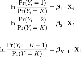
One fairly simple way to arrive at the multinomial logit model is to imagine, for K possible outcomes, running K-1 independent binary logistic regression models, in which one outcome is chosen as a "pivot" and then the other K-1 outcomes are separately regressed against the pivot outcome. This would proceed as follows, if outcome K (the last outcome) is chosen as the pivot:

$\begin{align} \ln \frac{\Pr(Y_i=1)}{\Pr(Y_i=K)} &= \boldsymbol\beta_1 \cdot \mathbf{X}_i \\ \ln \frac{\Pr(Y_i=2)}{\Pr(Y_i=K)} &= \boldsymbol\beta_2 \cdot \mathbf{X}_i \\ \cdots & \cdots \\ \ln \frac{\Pr(Y_i=K-1)}{\Pr(Y_i=K)} &= \boldsymbol\beta_{K-1} \cdot \mathbf{X}_i \\ \end{align}$

Note that we have introduced separate sets of regression coefficients, one for each possible outcome.

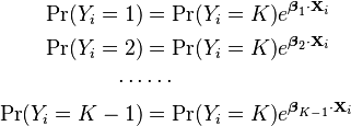
If we exponentiate both sides, and solve for the probabilities, we get:

$\begin{align} \Pr(Y_i=1) &= {\Pr(Y_i=K)}e^{\boldsymbol\beta_1 \cdot \mathbf{X}_i} \\ \Pr(Y_i=2) &= {\Pr(Y_i=K)}e^{\boldsymbol\beta_2 \cdot \mathbf{X}_i} \\ \cdots & \cdots \\ \Pr(Y_i=K-1) &= {\Pr(Y_i=K)}e^{\boldsymbol\beta_{K-1} \cdot \mathbf{X}_i} \\ \end{align}$

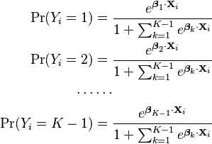
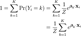
Using the fact that all K of the probabilities must sum to one, we find:

$\Pr(Y_i=K) = \frac{1}{1 + \sum_{k=1}^{K-1} e^{\boldsymbol\beta_k \cdot \mathbf{X}_i}}$

We can use this to find the other probabilities:

$\begin{align} \Pr(Y_i=1) &= \frac{e^{\boldsymbol\beta_1 \cdot \mathbf{X}_i}}{1 + \sum_{k=1}^{K-1} e^{\boldsymbol\beta_k \cdot \mathbf{X}_i}} \\ \Pr(Y_i=2) &= \frac{e^{\boldsymbol\beta_2 \cdot \mathbf{X}_i}}{1 + \sum_{k=1}^{K-1} e^{\boldsymbol\beta_k \cdot \mathbf{X}_i}} \\ \cdots & \cdots \\ \Pr(Y_i=K-1) &= \frac{e^{\boldsymbol\beta_{K-1} \cdot \mathbf{X}_i}}{1 + \sum_{k=1}^{K-1} e^{\boldsymbol\beta_k \cdot \mathbf{X}_i}} \\ \end{align}$

The fact that we run multiple regressions reveals why the model relies on the assumption of independence of irrelevant alternatives described above.

Estimating the coefficients

The unknown parameters in each vector β_k are typically jointly estimated by maximum a posteriori (MAP) estimation, which is an extension of maximum likelihood using regularization of the weights to prevent pathological solutions (usually a squared regularizing function, which is equivalent to placing a zero-mean Gaussian prior distribution on the weights, but other distributions are also possible). The solution is typically found using an iterative procedure such as generalized iterative scaling, iteratively reweighted least squares (IRLS), by means of gradient-based optimization algorithms such as L-BFGS, or by specialized coordinate descent algorithms.

As a log-linear model

The formulation of binary logistic regression as a log-linear model can be directly extended to multi-way regression. That is, we model the logarithm of the probability of seeing a given output using the linear predictor as well as an additional normalization factor:

$\begin{align} \ln \Pr(Y_i=1) &= \boldsymbol\beta_1 \cdot \mathbf{X}_i - \ln Z \, \\ \ln \Pr(Y_i=2) &= \boldsymbol\beta_2 \cdot \mathbf{X}_i - \ln Z \, \\ \cdots & \cdots \\ \ln \Pr(Y_i=K) &= \boldsymbol\beta_K \cdot \mathbf{X}_i - \ln Z \, \\ \end{align}$

As in the binary case, we need an extra term $- \ln Z$ to ensure that the whole set of probabilities forms a probability distribution, i.e. so that they all sum to one:

$\sum_{k=1}^{K} \Pr(Y_i=k) = 1$

The reason why we need to add a term to ensure normalization, rather than multiply as is usual, is because we have taken the logarithm of the probabilities. Exponentiating both sides turns the additive term into a multiplicative factor, and in the process shows why we wrote the term in the form $- \ln Z$ rather than simply $+ Z$:

$\begin{align} \Pr(Y_i=1) &= \frac{1}{Z} e^{\boldsymbol\beta_1 \cdot \mathbf{X}_i} \, \\ \Pr(Y_i=2) &= \frac{1}{Z} e^{\boldsymbol\beta_2 \cdot \mathbf{X}_i} \, \\ \cdots & \cdots \\ \Pr(Y_i=K) &= \frac{1}{Z} e^{\boldsymbol\beta_K \cdot \mathbf{X}_i} \, \\ \end{align}$

We can compute the value of Z by applying the above constraint that requires all probabilities to sum to 1:

$\begin{align} 1 = \sum_{k=1}^{K} \Pr(Y_i=k) &= \sum_{k=1}^{K} \frac{1}{Z} e^{\boldsymbol\beta_k \cdot \mathbf{X}_i} \\ &= \frac{1}{Z} \sum_{k=1}^{K} e^{\boldsymbol\beta_k \cdot \mathbf{X}_i} \\ \end{align}$

Therefore:

$Z = \sum_{k=1}^{K} e^{\boldsymbol\beta_k \cdot \mathbf{X}_i}$

Note that this factor is "constant" in the sense that it is not a function of Y_i, which is the variable over which the probability distribution is defined. However, it is definitely not constant with respect to the explanatory variables, or crucially, with respect to the unknown regression coefficients β_k, which we will need to determine through some sort of optimization procedure.

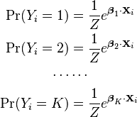
The resulting equations for the probabilities are

$\begin{align} \Pr(Y_i=1) &= \frac{e^{\boldsymbol\beta_1 \cdot \mathbf{X}_i}}{\sum_{k=1}^{K} e^{\boldsymbol\beta_k \cdot \mathbf{X}_i}} \, \\ \Pr(Y_i=2) &= \frac{e^{\boldsymbol\beta_2 \cdot \mathbf{X}_i}}{\sum_{k=1}^{K} e^{\boldsymbol\beta_k \cdot \mathbf{X}_i}} \, \\ \cdots & \cdots \\ \Pr(Y_i=K) &= \frac{e^{\boldsymbol\beta_K \cdot \mathbf{X}_i}}{\sum_{k=1}^{K} e^{\boldsymbol\beta_k \cdot \mathbf{X}_i}} \, \\ \end{align}$

Or generally:

$\Pr(Y_i=c) = \frac{e^{\boldsymbol\beta_c \cdot \mathbf{X}_i}}{\sum_{k=1}^{K} e^{\boldsymbol\beta_k \cdot \mathbf{X}_i}}$

The following function:

$\operatorname{softmax}(k,x_1,\ldots,x_n) = \frac{e^{x_k}}{\sum_{i=1}^n e^{x_i}}$

is referred to as the softmax function. The reason is that the effect of exponentiating the values $x_1,\ldots,x_n$ is to exaggerate the differences between them. As a result, $\operatorname{softmax}(k,x_1,\ldots,x_n)$ will return a value close to 0 whenever $x_k$ is significantly less than the maximum of all the values, and will return a value close to 1 when applied to the maximum value, unless it is extremely close to the next-largest value. Thus, the softmax function can be used to construct a weighted average that behaves as a smooth function (which can be conveniently differentiated, etc.) and which approximates the indicator function

$f(k) = \begin{cases} 1 \; \textrm{ if } \; k = \operatorname{\arg\max}(x_1, \ldots, x_n), \\ 0 \; \textrm{ otherwise}. \end{cases}$

Thus, we can write the probability equations as

$\Pr(Y_i=c) = \operatorname{softmax}(c, \boldsymbol\beta_1 \cdot \mathbf{X}_i, \ldots, \boldsymbol\beta_K \cdot \mathbf{X}_i)$

The softmax function thus serves as the equivalent of the logistic function in binary logistic regression.

Note that not all of the $\beta_k$ vectors of coefficients are uniquely identifiable. This is due to the fact that all probabilities must sum to 1, making one of them completely determined once all the rest are known. As a result there are only $k-1$ separately specifiable probabilities, and hence $k-1$ separately identifiable vectors of coefficients. One way to see this is to note that if we add a constant vector to all of the coefficient vectors, the equations are identical:

$\begin{align} \frac{e^{(\boldsymbol\beta_c + C) \cdot \mathbf{X}_i}}{\sum_{k=1}^{K} e^{(\boldsymbol\beta_k + C) \cdot \mathbf{X}_i}} &= \frac{e^{\boldsymbol\beta_c \cdot \mathbf{X}_i} e^{C \cdot \mathbf{X}_i}}{\sum_{k=1}^{K} e^{\boldsymbol\beta_k \cdot \mathbf{X}_i} e^{C \cdot \mathbf{X}_i}} \\ &= \frac{e^{C \cdot \mathbf{X}_i} e^{\boldsymbol\beta_c \cdot \mathbf{X}_i}}{e^{C \cdot \mathbf{X}_i} \sum_{k=1}^{K} e^{\boldsymbol\beta_k \cdot \mathbf{X}_i}} \\ &= \frac{e^{\boldsymbol\beta_c \cdot \mathbf{X}_i}}{\sum_{k=1}^{K} e^{\boldsymbol\beta_k \cdot \mathbf{X}_i}} \end{align}$

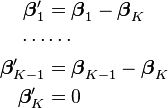
As a result, it is conventional to set $C = -\boldsymbol\beta_K$ (or alternatively, one of the other coefficient vectors). Essentially, we set the constant so that one of the vectors becomes 0, and all of the other vectors get transformed into the difference between those vectors and the vector we chose. This is equivalent to "pivoting" around one of the K choices, and examining how much better or worse all of the other K-1 choices are, relative to the choice are pivoting around. Mathematically, we transform the coefficients as follows:

$\begin{align} \boldsymbol\beta'_1 &= \boldsymbol\beta_1 - \boldsymbol\beta_K \\ \cdots & \cdots \\ \boldsymbol\beta'_{K-1} &= \boldsymbol\beta_{K-1} - \boldsymbol\beta_K \\ \boldsymbol\beta'_K &= 0 \end{align}$

This leads to the following equations:

$\begin{align} \Pr(Y_i=1) &= \frac{e^{\boldsymbol\beta'_1 \cdot \mathbf{X}_i}}{1 + \sum_{k=1}^{K-1} e^{\boldsymbol\beta'_k \cdot \mathbf{X}_i}} \, \\ \cdots & \cdots \\ \Pr(Y_i=K-1) &= \frac{e^{\boldsymbol\beta'_{K-1} \cdot \mathbf{X}_i}}{1 + \sum_{k=1}^{K-1} e^{\boldsymbol\beta'_k \cdot \mathbf{X}_i}} \, \\ \Pr(Y_i=K) &= \frac{1}{1 + \sum_{k=1}^{K-1} e^{\boldsymbol\beta'_k \cdot \mathbf{X}_i}} \, \\ \end{align}$

Other than the prime symbols on the regression coefficients, this is exactly the same as the form of the model described above, in terms of K-1 independent two-way regressions.

As a latent-variable model

It is also possible to formulate multinomial logistic regression as a latent variable model, following the two-way latent variable model described for binary logistic regression. This formulation is common in the theory of discrete choice models, and makes it easier to compare multinomial logistic regression to the related multinomial probit model, as well as to extend it to more complex models.

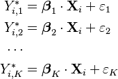
Imagine that, for each data point i and possible outcome k, there is a continuous latent variable Y_i,k^* (i.e. an unobserved random variable) that is distributed as follows:

$\begin{align} Y_{i,1}^{\ast} &= \boldsymbol\beta_1 \cdot \mathbf{X}_i + \varepsilon_1 \, \\ Y_{i,2}^{\ast} &= \boldsymbol\beta_2 \cdot \mathbf{X}_i + \varepsilon_2 \, \\ \cdots & \\ Y_{i,K}^{\ast} &= \boldsymbol\beta_K \cdot \mathbf{X}_i + \varepsilon_K \, \\ \end{align}$

where $\varepsilon_k \sim \operatorname{EV}_1(0,1),$ i.e. a standard type-1 extreme value distribution.

This latent variable can be thought of as the utility associated with data point i choosing outcome k, where there is some randomness in the actual amount of utility obtained, which accounts for other unmodeled factors that go into the choice. The value of the actual variable $Y_i$ is then determined in a non-random fashion from these latent variables (i.e. the randomness has been moved from the observed outcomes into the latent variables), where outcome k is chosen if and only if the associated utility (the value of $Y_{i,k}^{\ast}$) is greater than the utilities of all the other choices, i.e. if the utility associated with outcome k is the maximum of all the utilities. (Since the latent variables are continuous, the probability of two having exactly the same value is 0, so we basically don't have to worry about that situation.) That is:

$\begin{align} \Pr(Y_i = 1) &= \Pr(Y_{i,1}^{\ast} > Y_{i,2}^{\ast} \text{ and } Y_{i,1}^{\ast} > Y_{i,3}^{\ast}\text{ and } \cdots \text{ and } Y_{i,1}^{\ast} > Y_{i,K}^{\ast}) \\ \Pr(Y_i = 2) &= \Pr(Y_{i,2}^{\ast} > Y_{i,1}^{\ast} \text{ and } Y_{i,2}^{\ast} > Y_{i,3}^{\ast}\text{ and } \cdots \text{ and } Y_{i,2}^{\ast} > Y_{i,K}^{\ast}) \\ \cdots & \\ \Pr(Y_i = K) &= \Pr(Y_{i,K}^{\ast} > Y_{i,1}^{\ast} \text{ and } Y_{i,K}^{\ast} > Y_{i,2}^{\ast}\text{ and } \cdots \text{ and } Y_{i,K}^{\ast} > Y_{i,K-1}^{\ast}) \\ \end{align}$

Or equivalently:

$\begin{align} \Pr(Y_i = 1) &= \Pr(\max(Y_{i,1}^{\ast},Y_{i,2}^{\ast},\ldots,Y_{i,K}^{\ast})=Y_{i,1}^{\ast}) \\ \Pr(Y_i = 2) &= \Pr(\max(Y_{i,1}^{\ast},Y_{i,2}^{\ast},\ldots,Y_{i,K}^{\ast})=Y_{i,2}^{\ast}) \\ \cdots & \\ \Pr(Y_i = K) &= \Pr(\max(Y_{i,1}^{\ast},Y_{i,2}^{\ast},\ldots,Y_{i,K}^{\ast})=Y_{i,K}^{\ast}) \\ \end{align}$

Let's look more closely at the first equation, which we can write as follows:

$\begin{align} \Pr(Y_i = 1) &= \Pr(Y_{i,1}^{\ast} > Y_{i,k}^{\ast}\ \forall\ k=2,\ldots,K) \\ &= \Pr(Y_{i,1}^{\ast} - Y_{i,k}^{\ast} > 0\ \forall\ k=2,\ldots,K) \\ &= \Pr(\boldsymbol\beta_1 \cdot \mathbf{X}_i + \varepsilon_1 - (\boldsymbol\beta_k \cdot \mathbf{X}_i + \varepsilon_k) > 0\ \forall\ k=2,\ldots,K) \\ &= \Pr((\boldsymbol\beta_1 - \boldsymbol\beta_k) \cdot \mathbf{X}_i > \varepsilon_k - \varepsilon_1\ \forall\ k=2,\ldots,K) \end{align}$

There are a few things to realize here:

1. In general, if $X \sim \operatorname{EV}_1(a,b)$ and $Y \sim \operatorname{EV}_1(a,b)$ then $X - Y \sim \operatorname{Logistic}(0,b).$ That is, the difference of two independent identically distributed extreme-value-distributed variables follows the logistic distribution, where the first parameter is unimportant. This is understandable since the first parameter is a location parameter, i.e. it shifts the mean by a fixed amount, and if two values are both shifted by the same amount, their difference remains the same. This means that all of the relational statements underlying the probability of a given choice involve the logistic distribution, which makes the initial choice of the extreme-value distribution, which seemed rather arbitrary, somewhat more understandable.
2. The second parameter in an extreme-value or logistic distribution is a scale parameter, such that if $X \sim \operatorname{Logistic}(0,1)$ then $bX \sim \operatorname{Logistic}(0,b).$ This means that the effect of using an error variable with an arbitrary scale parameter in place of scale 1 can be compensated simply by multiplying all regression vectors by the same scale. Together with the previous point, this shows that the use of a standard extreme-value distribution (location 0, scale 1) for the error variables entails no loss of generality over using an arbitrary extreme-value distribution. In fact, the model is nonidentifiable (no single set of optimal coefficients) if the more general distribution is used.
3. Because only differences of vectors of regression coefficients are used, adding an arbitrary constant to all coefficient vectors has no effect on the model. This means that, just as in the log-linear model, only K-1 of the coefficient vectors are identifiable, and the last one can be set to an arbitrary value (e.g. 0).

Actually finding the values of the above probabilities is somewhat difficult, and is a problem of computing a particular order statistic (the first, i.e. maximum) of a set of values. However, it can be shown that the resulting expressions are the same as in above formulations, i.e. the two are equivalent.

Estimation of intercept

When using multinomial logistic regression, one category of the dependent variable is chosen as the reference category. Separate odds ratios are determined for all independent variables for each category of the dependent variable with the exception of the reference category, which is omitted from the analysis. The exponential beta coefficient represents the change in the odds of the dependent variable being in a particular category vis-a-vis the reference category, associated with a one unit change of the corresponding independent variable.

Application in natural language processing

In natural language processing, multinomial LR classifiers are commonly used as an alternative to naive Bayes classifiers because they do not assume statistical independence of the random variables (commonly known as features) that serve as predictors. However, learning in such a model is slower than for a naive Bayes classifier, and thus may not be appropriate given a very large number of classes to learn. In particular, learning in a Naive Bayes classifier is a simple matter of counting up the number of co-occurrences of features and classes, while in a maximum entropy classifier the weights, which are typically maximized using maximum a posteriori (MAP) estimation, must be learned using an iterative procedure; see #Estimating the coefficients.

See also

• Logistic regression
• Multinomial probit