Variance decomposition of forecast errors

In econometrics and other applications of multivariate time series analysis, a variance decomposition or forecast error variance decomposition (FEVD) is used to aid in the interpretation of a vector autoregression (VAR) model once it has been fitted.^[1] The variance decomposition indicates the amount of information each variable contributes to the other variables in the autoregression. It determines how much of the forecast error variance of each of the variables can be explained by exogenous shocks to the other variables.

Calculating the forecast error variance

For the VAR (p) of form

y_t=\nu +A_1y_{t-1}+\dots+A_p y_{t-p}+u_t

.

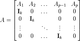
This can be changed to a VAR(1) structure by writing it in companion form (see general matrix notation of a VAR(p))

Y_t=V+A Y_{t-1}+U_t

where

A=\begin{bmatrix} A_1 & A_2 & \dots & A_{p-1} & A_p \\ \mathbf{I}_k & 0 & \dots & 0 & 0 \\ 0 & \mathbf{I}_k & & 0 & 0 \\ \vdots & & \ddots & \vdots & \vdots \\ 0 & 0 & \dots & \mathbf{I}_k & 0 \\ \end{bmatrix}

,

Y=\begin{bmatrix} y_1 \\ \vdots \\ y_p \end{bmatrix}

,

V=\begin{bmatrix} \nu \\ 0 \\ \vdots \\ 0 \end{bmatrix}

and

U_t=\begin{bmatrix} u_t \\ 0 \\ \vdots \\ 0 \end{bmatrix}

where $y_t$ , $\nu$ and $u$ are $k$ dimensional column vectors, $A$ is $kp$ by $kp$ dimensional matrix and $Y$ , $V$ and $U$ are $kp$ dimensional column vectors.

The mean squared error of the h-step forecast of variable j is

\mathbf{MSE}[y_{j,t}(h)]=\sum_{i=0}^{h-1}\sum_{k=1}^{K}(e_j'\Theta_ie_k)^2=\bigg(\sum_{i=0}^{h-1}\Theta_i\Theta_i'\bigg)_{jj}=\bigg(\sum_{i=0}^{h-1}\Phi_i\Sigma_u\Phi_i'\bigg)_{jj},

and where

$e_j$ is the j^th column of $I_K$ and the subscript $jj$ refers to that element of the matrix

$\Theta_i=\Phi_i P ,$ where $P$ is a lower triangular matrix obtained by a Cholesky decomposition of $\Sigma_u$ such that $\Sigma_u = PP'$ , where $\Sigma_u$ is the covariance matrix of the errors $u_t$