presentation
 Omar Ameur
visibility
…
description
19 pages
link
1 file
Sign up for access to the world's latest research
checkGet notified about relevant papers
checkSave papers to use in your research
checkJoin the discussion with peers
checkTrack your impact
AI-generated Abstract
This paper presents a formal proof of stability for a piecewise affine system (PWA) affected by friction, showcasing its asymptotic stability through the identification of an appropriate Lyapunov function. The approach allows for convergence not only to a point but to a broader equilibrium set, extending previous methodologies and demonstrating less conservatism in the resultant stability analysis.
Figures (12)


Related papers
Existence of piecewise linear Lyapunov functions in arbitrary dimensions
Discrete and Continuous Dynamical Systems, 2012
Lyapunov functions are an important tool to determine the basin of attraction of exponentially stable equilibria in dynamical systems. In Marinosson (2002), a method to construct Lyapunov functions was presented, using finite differences on finite elements and thus transforming the construction problem into a linear programming problem. In Hafstein (2004), it was shown that this method always succeeds in constructing a Lyapunov function, except for a small, given neighbourhood of the equilibrium. For two-dimensional systems, this local problem was overcome by choosing a fan-like triangulation around the equilibrium. In Giesl/Hafstein (2010) the existence of a piecewise linear Lyapunov function was shown, and in Giesl/Hafstein (subm.) it was shown that the above method with a fan-like triangulation always succeeds in constructing a Lyapunov function, without any local exception. However, the previous papers only considered two-dimensional systems. This paper generalises the existence of piecewise linear Lyapunov functions to arbitrary dimensions.
On Liapunov functions for nonautonomous systems
Journal of Mathematical Analysis and Applications, 1974
Discontinuous piecewise quadratic Lyapunov functions for planar piecewise affine systems
Journal of Mathematical Analysis and Applications, 2013
This article appeared in a journal published by Elsevier. The attached copy is furnished to the author for internal non-commercial research and education use, including for instruction at the authors institution and sharing with colleagues. Other uses, including reproduction and distribution, or selling or licensing copies, or posting to personal, institutional or third party websites are prohibited. In most cases authors are permitted to post their version of the article (e.g. in Word or Tex form) to their personal website or institutional repository. Authors requiring further information regarding Elsevier's archiving and manuscript policies are encouraged to visit:
A constructive converse Lyapunov theorem on exponential stability
Discrete and Continuous Dynamical Systems, 2004
Closed physical systems eventually come to rest, the reason being that due to friction of some kind they continuously lose energy. The mathematical extension of this principle is the concept of a Lyapunov function. A Lyapunov function for a dynamical system, of which the dynamics are modelled by an ordinary differential equation (ODE), is a function that is decreasing along any trajectory of the system and with exactly one local minimum. This implies that the system must eventually come to rest at this minimum. Although it has been known for over 50 years that the asymptotic stability of an ODE's equilibrium is equivalent to the existence of a Lyapunov function for the ODE, there has been no constructive method for non-local Lyapunov functions, except in special cases. Recently, a novel method to construct Lyapunov functions for ODEs via linear programming was presented [5], , which includes an algorithmic description of how to derive a linear program for a continuous autonomous ODE, such that a Lyapunov function can be constructed from any feasible solution of this linear program. We will show how to choose the free parameters of this linear program, dependent on the ODE in question, so that it will have a feasible solution if the equilibrium at the origin is exponentially stable. This leads to the first constructive converse Lyapunov theorem in the theory of dynamical systems/ODEs. 1991 Mathematics Subject Classification. 93D05, 93D20, 93D30, 34D05, 34D20.
Existence of piecewise affine Lyapunov functions in two dimensions
Journal of Mathematical Analysis and Applications, 2010
In [10] a method to compute Lyapunov functions for systems with asymptotically stable equilibria was presented. The method uses finite differences on finite elements to generate a linear programming problem for the system in question, of which every feasible solution parameterises a piecewise affine Lyapunov function. In it was proved that the method always succeeds in generating a Lyapunov function for systems with an exponentially stable equilibrium. However, the proof could not guarantee that the generated function has negative orbital derivative locally in a small neighborhood of the equilibrium. In this article we give an example of a system, where no piecewise affine Lyapunov function with the proposed triangulation scheme exists. This failure is due to the triangulation of the method being too coarse at the equilibrium, and we suggest a fan-like triangulation around the equilibrium. We show that for any two-dimensional system with an exponentially stable equilibrium there is a local triangulation scheme such that the system possesses a piecewise affine Lyapunov function. Hence, the method might eventually be equipped with an improved triangulation scheme that does not have deficits locally at the equilibrium.
Explicit Stability Conditions for Continuous Systems
Lecture Notes in Control and Information Sciences, 2005
Regions of stability for limit cycles of piecewise linear systems
2003
This paper starts by presenting local stability conditions for limit cycles of piecewise linear systems (PLS), based on analyzing the linear part of Poincaré maps. Local stability guarantees the existence of an asymptotically stable neighborhood around the limit cycle. However, tools to characterize such neighborhood do not exist. This work gives conditions in the form of LMIs that guarantee asymptotic stability of PLS in a reasonably large region around a limit cycle, based on recent results on impact maps and surface Lyapunov functions (SuLF). These are exemplified with a biological application: a 4 th -order neural oscillator, also used in many robotics applications like, for example, juggling and locomotion.
Stability of controlled motion
Journal of Mathematical Analysis and Applications, 1969
Stability of Dynamical Systems: a Constructive Approach
IEEE Transactions on Circuits and Systems, 1979
A piecewise affine approach to the analysis of the
stability of the electro-pneumatic systems
Omar AMEUR
Paolo MASSIONI, Gérard SCORLETTI,
Xavier BRUN and Mohamed SMAOUI
Laboratoire Ampère,
UMR 5005
Lyon, France
CDC, December 2014
1 / 19
Contents
1
Introduction
Motivation
Stick slip problem
2
Stability analysis
Piecewise affine systems
Contribution
Sketch of proof
Lyapunov function level curves
Lyapunov function evolution
3
Conclusions
2 / 19
Motivation: Fluid Power
Electro-pneumatic systems in industry studied at our laboratory
qmP
Chamber P
guiding rails
qmN
Chamber N
load
Non-linear dynamics
A major problem: the stick slip phenomenon
Pragmatic solution based on switched controllers [Turki et al. 2011]
Open problem: formal stability proof
3 / 19
Stick-Slip
qmP
Chamber P
guiding rails
qmN
Chamber N
load
=⇒ jerky movements
of the load (due to friction)
4 / 19
Stick-Slip
qmP
load
Chamber N
ey (m)
Chamber P
guiding rails
qmN
Time (s)
Pressures (Pa)
Why?
uncontrolled pressure
dynamics after stop
Stick-slip
Stick-slip
Stick-slip
Time (s)
5 / 19
Stick-Slip
Proposed solution [Turki et al. 2011]
Switching between two control laws:
(#1) dynamic regime law (trajectory tracking control,feedback linearisation )
(#2) static regime law (pressure control, feedback linearisation)
#1 #2 #1
#2
#1
#2
0.25
position [m]
0.2
0.15
0.1
0.05
0
rod position
reference
−0.05
0
0.5
1
1.5
2
2.5
3
3.5
4
4.5
5
t [s]
6 / 19
Stick-Slip
Proposed solution [Turki et al. 2011]
Switching between two control laws:
(#1) dynamic regime law (trajectory tracking control, feedback linearisation )
(#2) static regime law (pressure control, feedback linearisation)
#1
#2
State space
Friction model
Control law + friction =⇒ Piecewise affine system (PWA)
7 / 19
Piecewise affine systems
for x ∈ Xi ⊂ Rn
ẋ (t ) = Ai x (t ) + ai
X1
ey
ε1
0
X6
X4
X0
X5
X3
-ε1
X2
-ε
-ε2 ε2
ε
v
The aim
Formal proof of stability
Convergence to a neighborhood of reference position (convergence to an
equilibrium set)
8 / 19
Stability
Method (Classical case)
find a quadratic Lyapunov function V(x) (energy function)
Asymptotic stability
V (x ) > 0
V̇ (x ) < 0
Assess decay rate α
V̇ (x ) < −2αV (x )
=⇒ V (x ) < V (0) exp(−2αt )
9 / 19
Convergence to an equilibrium set
Finding a piecewise quadratic Lyapunov function
Continuous
especially on the boundary
Valid Lyapunov function
Allowing an equilibrium set Eeq
(instead of a point)
projection to the stable subspace
X1
ε1
ey
Vi (x ) > 0, x ∈ Xi \ Eeq
V̇i (x ) < 0, x ∈ Xi \ Eeq
V̇i (x ) = 0, x ∈ Eeq ⊂ X0 .
0
X6
X4
X0
X5
X3
-ε1
X2
-ε
-ε2 ε2
ε
v
10 / 19
Theorem [Ameur et al. CDC 2014]
Find:
U, W ∈ Rli ×li and T i , T ′i ∈ Rli with non-negative entries;
P i ∈ R(n+1)×(n+1) for 1 ≤ i ≤ N − 1, P 0 ∈ Rn×n and Lij ∈ R(n+1)×p
such that:
T
P j = P i + E ij LTij + Lij E ij , for (i , j ) ∈ Γij
(1)
ΠT AT0 P 0 Z1 = 0
(2)
and the following LMIs hold:
(
P0 ≻ 0
ΠT (AT0 P 0 + P 0 A0 )Π + 2αΠT P 0 Π ≺ 0
P i − Qi (T ′ ) − E T W i E i ≻ 0
i
i
AT P + P A + Q (T ) + E T U E + 2αP ≺ 0
i
i i
i
i
i i
i
i
i
=⇒ exponentially convergence to Eeq .
(3)
(4)
11 / 19
Contribution
Extending the former methods [Johanson & Rantzer 1998], [Hassibi & Boyd
1998],...
convergence to the set (not only origin)
The theorem in [Johanson & Rantzer 1998], is a special case of our Theorem for
Eeq = {0}
Ti = 0
α=0
The theorem in [Hassibi & Boyd 1998], is a special case of our Theorem for
Eeq = {0}
Ui = 0
α=0
Less conservatism than both former methods
12 / 19
Sketch of proof
Vi (x ) =
T
x
x
for x ∈ Xi , 1 ≤ i ≤ N − 1
Pi
1
1
Continuity
x
=0
On the boundary: E ij
1
then:
T
P j = P i + E ij LTij + Lij E ij =⇒
Valid Lyapunov function
T T
x
x
x
x
Pj
Pi
=
1
1
1
1
for x ∈ X0 (cell including equilibrium set)
V0 (x ) > 0, x ∈ X0 \ Eeq
P0 ≻ 0
T T
Π (A0 P 0 + P 0 A0 )Π + 2αΠT P 0 Π ≺ 0 ⇒
V̇0 (x ) < −2αV0 (ΠΠT x ), x ∈ X0 \ Eeq
T T
Π A0 P 0 Z 1 = 0
V̇0 (x ) = 0, x ∈ Eeq
13 / 19
Sketch of proof
Valid Lyapunov function
for x ∈ Xi , 1 ≤ i ≤ N − 1 (cell not including equilibrium set)
Vi (x ) > 0, x ∈ Xi
P i − Qi (T ′i ) − E Ti W i E i ≻ 0
⇒
AT P + P A + Q (T ) + E T U E + 2αP ≺ 0
i
i
i
V̇i (x ) < −2αVi (x ), x ∈ Xi
i
i i
i i
i
i
when
T
x
x
T
W
E
E
≥0
i i
i
1
1
T
x Qi (T ′i ) x ≥ 0
1
1
14 / 19
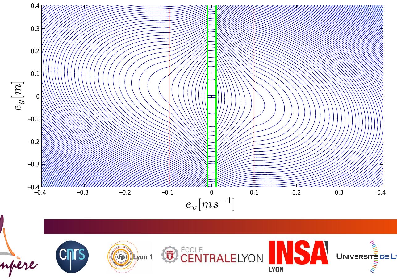
Lyapunov function level curves
Results of optimization under LMIs constraints (using Matlab/Yalmip/Sedumi)
0.4
0.3
0.2
ey [m]
0.1
0
−0.1
−0.2
−0.3
−0.4
−0.4
−0.3
−0.2
−0.1
0
0.1
0.2
0.3
0.4
ev [ms−1 ]
15 / 19
Lyapunov function evolution
γ : decay rate −→ γ ≥ α (Matlab: α = 0.49)
16 / 19
Conclusions and work in progress
Conclusion
General stability analysis method for piecewise affine systems with
equilibrium on a set
Solution to an open problem in fluid power (stability analysis of control laws to
avoid stick-slip problem)
Success story of theory and practice working together!!
Similar problems in power system control
Work in progress
Robustness analysis, tracking performance
17 / 19
Thank you for your attention
18 / 19
Tracking performance (vd 6= 0)
19 / 19