The Multi-Handler Knapsack Problem under Uncertainty

Introduction

The increasing competition due to both globalization of production processes and the movement of large quantities of freight between continents and countries creates the need for new tools for strategic and tactical decisions, that are able to deal with the stochastic nature of the processes involved. While this leads to new location and transportation problems [1,2], only a few studies deal with the stochastic study of packing problems [3]. This is mainly due to the peculiarities of the literature related to packing. In fact, even if packing problems play a central role in transportation and logistics, the problems presented in the literature are mainly related to operational issues [4,5]. Moreover, the parameter uncertainty affecting the final solutions such as the profit associated to item delivery or the cost of container renting is usually more evident in the planning phases rather than in the operational ones.

In this paper we introduce a new stochastic variant of the knapsack problem, the Multi-Handler Knapsack Problem under Uncertainty (MHKP u ). Given a set of items, characterized by volume and random profit, and a set of potential logistics handlers, the problem consists in finding a subset of items which maximizes the expected total profit. The profit is given by the sum of a deterministic profit and a stochastic profit oscillation, with unknown probability distribution, due to the random handling costs of the handlers.

A large number of real-life situations can be satisfactorily modeled as a MHKP u , e.g. in financial and resource allocation. The general idea is to think of the capacity of the knapsack as the available amount of a resource (i.e. budget) and the items as activities to which this resource can be allocated (i.e. shares). Moreover, these items present profits which are random variables. The MHKP u may also appear as a subproblem of larger optimization problems.

A specific application of the MHKP u can be found in the automotive sector [6]. There the delivery of cars from manufacturers to dealers is not managed by the manufacturers themselves, but is delegated to specialized companies. These companies manage both the finishing operations on the cars (e.g. removal of the protective wax, installation of specific accessories, etc.) and the logistics operations linked to delivery to the dealers. In order to have a more flexible structure, the fleet of auto-carriers used to deliver the cars is only partially owned by each company, while a substantial part of the deliveries is sub-contracted to micro-companies with highly variable random costs. Moreover, the auto-carriers have different capacities due to the presence of specific technical features. From the point of view of the cars that must be delivered, the net profit for the company is affected by different factors, including delays in the finishing operations, additional costs due to violations of the negotiated deadlines or additional transportation costs.

Another example of real-world applications of the MHKP u comes from trans-continental naval shipping operations, where freight transportation from eastern ports to Europe and North America is managed by specialized companies. The competition between the transportation companies, as well as the possibility of managing the port cranes by different operators, force the companies to consider both the profit given by the shipped items and the additional costs due to the logistics operations.

The problem can be also seen as a relaxation of container loading problems where the capacity of the given containers are collapsed into one single container. This leads to an approximation of the real problem suitable in strategic and tactical planning, where the stochastic nature of the profits in more relevant than the actual loading of the items. Moreover, it is required to obtain accurate solutions within a limited computational effort in order to explore multiple scenarios of the underlying business model.

Other applications come from the domain of Smart City and City Logistics, and particularly in the last mile delivery. One of the trends is to substitute traditional single-echelon routing structures with two and three-echelon ones. The reason is the willingness to use ''green'' vehicles inside the city, whilst consolidating the freight in medium and small sized transshipment depots, called satellites [7,8,9]. In the satellites different sequences of consolidation operations are done by different workers. The different skill levels of the workers can cause delay in the operations reducing the overall profit. A similar problem is present in yard management, where the profit oscillations are given by the operations done by workers working for yard management companies, different in skills and reliability.

In general, the MHKP u arises in logistics and production scheduling applications, where a single item can be managed by several handlers (third-party logistics providers or sub-contractors), whose costs affect the net profit of the item itself. The large number of possible handler cost scenarios and the difficulty to measure the associated handler costs suggest the representation of these net profits as stochastic variables with unknown probability distribution.

This paper introduces the formulation of the stochastic problem. From this formulation, a deterministic approximation is derived. In particular, under a mild hypothesis on the unknown probability distribution, the deterministic approximation becomes a knapsack problem where the total expected profit of the loaded items is proportional to the logarithm of the total accessibility of those items to the set of handlers. Moreover, at optimality, the percentage of an item handled by any handler is given by a multinomial Logit model. The paper is organized as follows. The literature review is introduced in Section 2. In Section 3 the model of the MHKP u is given. Section 4 is devoted to presenting the deterministic approximation of the MHKP u , while in Section 5 its two-stage program with fixed recourse is given. Finally, in Section 6 the deterministic approximation and the two-stage program with fixed recourse are tested and compared on a set of newly introduced instances. The conclusion of our work is reported in Section 7.

Literature review

While different variants of the stochastic knapsack problem are present in the literature, the MHKP u is absent. For this reason, we will consider some relevant literature on similar problems, highlighting the main differences with the problem faced in this paper.

A first group of studies consider deterministic profits and random volumes, with the goal of maximizing the total expected value of selected items, while ensuring that the probability to satisfy the knapsack capacity is limited by some upper bounds. Usually, heavy assumptions on the distribution of the random volumes are considered (e.g. [10], [11] where item volumes have a Bernoulli distribution, and [12], [13] where the distribution is a Normal one). These assumptions on the distributions heavily limit the possibility to extend the results to other variants of the problem.

A second group of studies deals with random profits and the goal to assign a set of items to the knapsack in order to maximize the probability of achieving some target total value. They are usually more related to financial and economic issues than to the impact of the operations on the final revenue [14,15,16]. Unfortunately, these problems differ from MHKP u because they consider the random profit associated only to the item, while in MHKP u the randomness is given by the interaction between the item and the handler managing the loading/unloading operations.

Finally, from a methodological point of view, the study most similar to the present paper is [3], where the authors consider the stochastic version of the Generalized Bin Packing Problem, a recently introduced packing problem where, given a set of bins characterized by volume and cost and a set of items characterized by volume and profit (which also depends on bins), a subset of items is selected for loading into a subset of bins which maximizes the total net profit, while satisfying the volume and bin availability constraints [17]. Similarly to MHKP u , the item profits are random variables and the probability distribution of these random variables is assumed to be unknown.

The MHKP u

In the MHKP u the item profits are random variables. In fact, they are composed by a deterministic profit plus a random term, which represents the profit oscillation due to the handling costs occurred by the different handlers for preparing items for loading. In practice, such profit oscillations randomly depend on the handling scenarios adopted by the handlers for preparing items for loading and are actually very difficult to be measured. This implies that the probability distribution of these random terms must be assumed as unknown.

Let it be The MHKP u is formulated as follows max {y,x} i∈I

The objective function (1) expresses the maximization of the profit of the items loaded into the knapsack plus the expected value of the handling profit; constraint (2) ensures that the capacity of the knapsack is not exceeded; constraints (3) guarantee that any item is completely processed by some handlers only if it is loaded. Finally, (4)-(5) are the integrality and non-negativity constraints, respectively.

Let us assume thatθ jl are independent and identically distributed (i.i.d.) random variables with a common and unknown probability distribution

Let us define withθ j the maximum of the random profit oscillationsθ jl for handler j among the alternative scenarios l ∈ Lθ j = max l∈Lθ jl j ∈ J.

Because F(x) is unknown,θ j is still of course a random variable with unknown probability distribution given by

As, for any handler j,θ j ≤ x ⇐⇒θ jl ≤ x, l ∈ L andθ jl are independent, using (6) one gets

We assume that the knapsack loading is efficiency-based so that, for any item i and any handler j, among the alternative scenarios l ∈ L the one which maximizes the random profitp i j (θ jl ) will be selected. This does not mean that, in the stochastic problem, we select the model scenario which maximizes the profit, but that, when the actual profits become known (e.g. in day-by-day operations, the profits of a given day), the choice among the different alternatives is done by taking the most profitable one.

Then, the random profit of item i when it is loaded (i.e. y i = 1) by handler j becomes

The maximum profit oscillationθ j can be either positive or negative, but, in practice, its absolute value does not overcome the profit p i j , so thatp i j (θ j ) is always non negative.

The expected maximum total profit of the loaded items is obtained by solving the following problem

The objective function (11) maximizes the expected total profit for the loaded items. Constraints (12) guarantee that each loaded item is completely processed by some handlers, while (13) are the non-negativity constraints.

For each item i, let us consider the handler j = i * (for the sake of simplicity, we assume it is unique), which gives the maximum random profit for loading the item.

The maximum random profit for loading item i then becomes

and the optimal variables x i j are

which satisfy (12) and (13). Using (14), (15), and the linearity of the expected value operator E, the objective function (11) becomes

The MHKP u (1)-(5) then becomes

However, the calculation ofp i in (18) requires to know the probability distribution of the maximum random profit for loading item i, i.e.p i (θ i * ) in (17), which will be derived in the next section.

The deterministic approximation of the MHKP u

By (10) and (14), let

be the probability distribution of the maximum random profit for loading item i. As, for any item i, max j∈J p i j +θ j ≤ x ⇐⇒ p i j +θ j ≤ x, j ∈ J, and the random variablesθ j are independent (becauseθ jl are independent), due to (8) and (9), G i {x} in (21) becomes a function of the total number |L| of handling scenarios for loading as follows

First, let us consider the following aspect: the optimal solution of problem (11)- (13) does not change if any arbitrary constant is added or subtracted to the random variablesθ j .

Let us choose this constant as the root a of the equation

Let us assume that |L| is large enough to use the asymptotic approximation lim |L|→+∞ G i (x, |L|) as a good approximation of G i (x), i.e.

The calculation of the limit in (24) would require to know the probability distribution F(.) in (6), which is still unknown. From [3], we know that under a mild assumption on the shape of the unknown probability distribution F(.) (i.e. it is asymptotically exponential in its right tail), the limit in (24) tends towards the following Gumbel [18] probability distribution

where β > 0 is a parameter to be calibrated and

is the accessibility, in the sense of Hansen [19], of item i to the set of handlers.

The accessibility in the sense of Hansen is defined as the potential of opportunities for interaction and is a measure of the intensity of the possibility of interaction. Here the interaction is between item and handlers. (26) shows that the accessibility of an item to the set of handlers is proportional to a function of profits associated to the different handlers.

Using the probability distribution G i (x) given by (25), after some manipulations,p i in (17) becomeŝ

subject to (19)- (20), where Φ = i∈I A y i i is the total accessibility of the loaded items to the set of handlers. It is interesting to observe that the total expected profit of the loaded items is proportional to the logarithm of the total accessibility of those items to the set of handlers.

In the following, we will refer to the deterministic approximation of the MHKP u as DA-MHKP u .

The following theorem holds Theorem 1. At optimality, the percentage of each item i handled by handler j, x i j , is given by

Proof. At optimality, the probability that item i is handled by handler j is equal to the probability that handler j is that one of maximum profit. Then, from the Total Probability Theorem [20], one obtains

where t = e −βx .

It is trivial to check for x i j the satisfaction of constraints (12) and (13).

Expression (29) represents a multinomial Logit model, which is widely used in choice theory [21]. In our case, it describes how the optimal handling of item i is split among different handlers j, due to the stochastic handling profit of item i.

The MHKP u as a two-stage program with fixed recourse

Approximating the profit stochasticity by discretizing the probability distributions and generating a set of scenarios S ⊆ L, the MHKP u (1)-(5) may be interpreted as a two-stage program with fixed recourse.

Let be the variables Moreover, we define by π +s i j = p i + p i j +θ js (31) and π −s i j = −π +s i j − π i j (32) the stochastic profits related to loading and unloading operations in the second stage, respectively, where −π i j represents an extra cost to be paid for unloading item i by handler j in the second stage. Finally, given the probability ρ s of each second-stage scenario s, the two-stage program with fixed recourse, named 2S-MHKP u , is formulated as follows max {y,x} i∈I p i y i + i∈I j∈J

x +s i j ≥ 0 i ∈ I, j ∈ J, s ∈ S (47)

The objective function (33) expresses the maximization of the total profit, given by the sum of the first stage profit plus the expected profit of the items handled in the second stage. Note that constraints (34) and (35) are the first stage constraints, while constraints (36)-(42) are the second stage ones. In particular, constraints (34) and (36) ensure that the capacity of the knapsack is not exceeded in first and second stages, respectively. Constraints (35) guarantee that any item is completely processed by some handlers only if it is loaded. Constraints (37) and (38) guarantee that if an item is loaded or unloaded in the second stage it is completely processed by some handlers. Constraints (39) establish that no item can be handled for loading in the second stage if it has already been loaded in the first stage. Similarly, constraints (40) establish that no item can be handled for unloading in the second stage if it has not been loaded in the first stage. Constraints (41) and (42) are the non-anticipativity constraints. Finally, constraints (43)-(45) and (46)-(48) are the integrality and the non-negativity constraints, respectively.

The optimal solutions of the two-stage model 2S-MHKP u and the deterministic approximation DA-MHKP u are strictly related. Let us suppose to have an optimal solution of model DA-MHKP u . This model gives us a feasible approximation of the first-stage variables y i , while it gives, by (29), a continuous relaxation of the assignment variables x i j . Notice that, given the values of the variables x i j in (29), one can derive a feasible first-stage solution of 2S-MHKP u by fixing to one, for each item with y i = 1, any x i j variable associated to it (for example, the one with the greatest value). This means that the information given by model DA-MHKP u is related to the first level only, while to obtain the possible recursion we need to force the first-level solution in the two-stage model.

Computational results

In this section, we present and analyze the results of the computational experiments. The first goal is to assess the behavior of the 2S-MHKP u , the two-stage program with fixed recourse for the MHKP u proposed. The second is to evaluate the effectiveness of the deterministic approximation of the MHKP u we derived. Moreover, we want to calculate and evaluate the handling costs obtained by using our approximated results as first-stage decisions of the 2S-MHKP u .

Generate p i and p i j according to [22] computep as the mean of p i + p i jθ j1 = D(θ js ; Kp/2, 0, Kp) The two-stage program with fixed recourse was implemented with CPLEX 12.3. Experiments were performed on a Intel i7 2 Ghz workstation with 6 GB of RAM. Section 6.1 introduces the instance set. The calibration of the deterministic approximation of the MHKP u is described in Section 6.2, whilst the comparison between the two-stage and approximated solutions is given in Section 6.3. Finally, we study the impact of the approximated results on the two-stage program with fixed recourse in Section 6.4.

Instance set

No instances are present in the literature for this stochastic version of the knapsack problem. We then generated instances, partially based on those available for the deterministic knapsack problem [22].

Instances were created with the goal of providing the means to explore the impact of both the correlation between volume and profit of the items and the different probability distributions of the profit oscillations. Thus, the instances are characterized by various correlation strengths, as well as different probability distributions. Ten instances were randomly generated for each combination of the parameters.

• Number of items in the interval [100, 1000].

• Number of handlers in the interval [3,5].

• Item volume uniformly distributed in the interval [1, R], where R = 1000.

• Deterministic item profits generated according to the following three rules UC: the deterministic item profits are uncorrelated to item volumes. They are uniformly generated in the interval [1, R] [5,22].

SC: the deterministic item profits are strongly correlated with the item volumes. The profit is defined as w i +R/10, where w i is the item volume [5,22].

PC: the deterministic item profits are proportionally correlated with the item volumes.The profit is defined as αw i , where α is uniformly drawn from the interval [1,5].

• Capacity of the knapsack was computed according to h H+1 i∈I w i , where H is the number of instances for a set of parameters and h ∈ [1, H] is the identification of an instance in that subset. This approach covers a large number of cases, diversifying the correlation between the parameters and the maximum capacity of the knapsack.

• Scenario generation. For each combination of the parameters described above, we first generate, for all the scenarios, the deterministic the item profits according to the above three rules. Given the average value of the deterministic profits, letp, let P K = Kp be the maximum profit oscillation, where K belongs to the set {0.1, 0.3, 0.5}. The item profit oscillations were generated asθ j|S | = D(θ js ; Kp/2, 0, Kp), where D(θ js ; µ, min, max) is the distribution D with mean µ and truncated between the values min and max (see Figure 1). In our tests we used the Uniform and the Gumbel distributions.

Figure 1

Having solved the instances 10 times each and computed the standard deviation and the mean of the optima over the runs, we derived that the appropriate number of scenarios is 50. For each instance, this value ensures a maximum ratio between the standard deviation and the mean for the optima which is less than 1%.

The parameters were also chosen to reflect realistic cases of supply chain applications. In details, the different levels of correlation between item volumes and profits have the double effect to explore more challenging instances from the computation point of view [22] and explore price policies quite common in transportation [23]. The interval of item volumes and their link to the knapsack capacity is derived from Pisinger [22]. Finally, the bound of the stochastic oscillations has been set as in Tadei et al. [2] and reflects typical boundaries for profit oscillations in logistics.

Calibration of the β parameter

The deterministic approximation of the MHKP u given by (28)

More sophisticated methods to calibrate β can be found in [24].

Comparison of two-stage program and deterministic approximation results

The two-stage program solutions showed a common trend: the 2S-MHKP u reserves half of the total knapsack capacity in the second stage. For this reason, no items are unloaded in 99% of the instances. This means that the 2S-MHKP u uses the knowledge given by the scenarios in order to forecast what items can be immediately loaded, while preserving a proper loading space for items to be arranged in the recourse. This leads to a drastic reduction of the unloading and rearranging operations. Thus, the 2S-MHKP u policy is quite far from the usual supply chain approach of almost fully loading the knapsack in advance, while the unloading/rearranging operations are made at a later time and the percentage gap with the optimal solution can easily overcome 10%.

Here we summarize the results for all instances and different combinations of the parameters. The performance, in terms of optimality gap, is defined by the relative percentage error of the approximated solution when compared to the optimum. Moreover, we estimate the solution likelihood as the percentage of items loaded by the approximated solution which are also present in the optimal solution.

Note that the comparison results do not consider the number of handlers, which does not seem to affect the average performance of the deterministic approximation. Table 1 reports the percentage optimality gap and the solution likelihood of the deterministic approximation for all combinations of the parameters, while varying the probability distribution (either Gumbel or Uniform). The first column displays the number of items, while Columns 2-3 and 5-6 report the mean and variance of the optimality gap, and Columns 4 and 7 show the mean percentage solution likelihood. The best mean values are obtained for the Gumbel distribution, that is very close to the optimum (0.12% for larger instances) and characterized by a negligible variance. Moreover, increasing the number of items gives better results for the deterministic approximation. Similarly, in terms of likelihood, this method guarantees results close to the optimum for both distributions. Table 2 reports the percentage optimality gap and the solution likelihood performance of the deterministic approximation while varying the correlation between profits and volumes of items (Column 2) and the probability distribution (Columns 3-8). The results indicate that the strongly correlated instances (SC) yield the worst gaps, as well as the worst solution likelihood, with an average optimality gap of about 0.27% and 1.54% for the Gumbel and the Uniform distributions, respectively. For uncorrelated instances (UC) and the Gumbel distribution, some solutions of the deterministic approximation exactly match the two-stage program solutions. The analysis of the impact of the maximum profit oscillations on the results accuracy is proposed in Table 3, considering different probability distributions (Columns 3-8). Recalling the definition of the maximum profit oscillation P K = Kp, column 2 represents the percentage K of the mean profitp of the instances. The gap and the solution likelihood are clearly inversely proportional to the range of the oscillations. Indeed, the best mean values are obtained for K = 0.1. In conclusion, the results are very promising. The procedure performs very well for all types of instances and distributions and guarantees a high accuracy. The best performance is obtained if the random profits have a Gumbel distribution, that is usually the case for real market oscillations. Moreover, the variance of the results is tight and in some cases close to zero. With respect to the solution likelihood, the mean values are all greater than 95% and increase according to the number of items.

Table 1

Optimality gap and solution likelihood of the deterministic approximation

Table 2

Optimality gap and solution likelihood for the profit correlation rules

Table 3

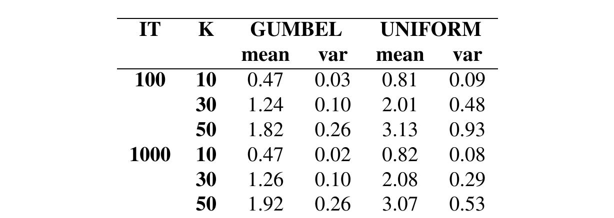
Optimality gap and solution likelihood for the maximum profit oscillations

As we expected, the mean optimality gap slightly increases for instances with Uniform distributed profit oscillations, but results are stable for each combination of the parameters and improve with respect to the number of items. Furthermore, it is interesting to note that the hardest subset of instances are the stronglly correlated ones. In fact, this kind of instance is characterized by a peculiar profit-volume correlation, as shown in [22].

From a computational point of view, the average CPU-times to solve to optimality the 2S-MHKP u and to compute the deterministic approximation are about 120 seconds and less than one second, respectively.

Usage of the approximated model as a decision tool

In the last part of this computational analysis, we analyze the losses, in terms of optimality gap, obtained by plugging the solution of the deterministic approximation of the MHKP u into the first-stage decision of the 2S-MHKP u [25]. In this way we can measure the accuracy of the approximated model when used not only as a method to calculate the optimum, but also as a decision tool to actually choose the items to be loaded. This means that the only degrees of freedom to maximize the objective function are the item-to-handler assignments and the handling operations in the second stage. Indeed, the effect of this strategy is the increase of the unloading operations, which does not exceed 6% of total operations, however.

Next, we present the comparison results organized as in Section 6.3. Tables 4, 5, and 6 summarize the average gap for all combinations of the parameters, for the profit correlations and for the maximum profit oscillations, respectively. As expected, the best performance is obtained by instances with the Gumbel distribution (Table 4). With respect to the profit correlations, the observed gap of SC instances is worse than other rules (Table 5). Finally, the gap increases according to the maximum range of the random profits (Table 6).

Table 4

Optimality gap with fixed first stage decision IT GUMBEL UNIFORM mean var mean var 100 1.18 0.44 1.99 1.40 1000 1.22 0.48 1.99 1.15

Table 5

Optimality gap with fixed first stage decision for the profit correlation rules

Table 6

Optimality gap with fixed first stage decision for the maximum profit oscillations

Conclusions

In this paper we have addressed the Multi-Handler Knapsack Problem under Uncertainty, which consists in finding a subset of items which maximizes the expected total profit, given by the sum of deterministic profits plus stochastic profit oscillations. One of the main features of this problem is that the profit oscillations are random variables with unknown probability distribution.

From a theoretical perspective, the paper shows that, under a mild assumption, the probability distribution of the maximum random profit for loading any item becomes a Gumbel distribution. Moreover, the total expected profit of the loaded items is proportional to the logarithm of the total accessibility of those items to the set of handlers and, at optimality, any item is handled by the set of handlers according to a multinomial Logit model. The deterministic approximation of the stochastic model obtained provides very promising results on a large set of instances in negligible computing time.

In conclusion, the performance of the methodology proposed is particularly good when the probability distribution of the random profits of the stochastic model is a Gumbel distribution, even if good results are also provided by the Uniform distribution. This feature makes our deterministic approximation a good predictive tool for considering stochastic handling costs in supply chain problems.