Arnoldi iteration

In numerical linear algebra, the Arnoldi iteration is an eigenvalue algorithm and an important example of iterative methods. Arnoldi finds the eigenvalues of general (possibly non-Hermitian) matrices; an analogous method for Hermitian matrices is the Lanczos iteration. The Arnoldi iteration was invented by W. E. Arnoldi in 1951.

The term iterative method, used to describe Arnoldi, can perhaps be somewhat confusing. Note that all general eigenvalue algorithms must be iterative. This is not what is referred to when we say Arnoldi is an iterative method. Rather, Arnoldi belongs to a class of linear algebra algorithms (based on the idea of Krylov subspaces) that give a partial result after a relatively small number of iterations. This is in contrast to so-called direct methods, which must complete to give any useful results.

Arnoldi iteration is a typical large sparse matrix algorithm: It does not access the elements of the matrix directly, but rather makes the matrix map vectors and makes its conclusions from their images. This is the motivation for building the Krylov subspace.

Krylov subspaces and the power iteration

An intuitive method for finding an eigenvalue (specifically the largest eigenvalue) of a given m × m matrix $A$ is the power iteration. Starting with an initial random vector b, this method calculates Ab, A²b, A³b,… iteratively storing and normalizing the result into b on every turn. This sequence converges to the eigenvector corresponding to the largest eigenvalue, $\lambda_{1}$. However, much potentially useful computation is wasted by using only the final result, $A^{n-1}b$. This suggests that instead, we form the so-called Krylov matrix:

$K_{n} = \begin{bmatrix}b & Ab & A^{2}b & \cdots & A^{n-1}b \end{bmatrix}.$

The columns of this matrix are not orthogonal, but in principle, we can extract an orthogonal basis, via a method such as Gram–Schmidt orthogonalization. The resulting vectors are a basis of the Krylov subspace, $\mathcal{K}_{n}$. We may expect the vectors of this basis to give good approximations of the eigenvectors corresponding to the $n$ largest eigenvalues, for the same reason that $A^{n-1}b$ approximates the dominant eigenvector.

The Arnoldi iteration

The process described above is intuitive. Unfortunately, it is also unstable. This is where the Arnoldi iteration enters.

The Arnoldi iteration uses the stabilized Gram–Schmidt process to produce a sequence of orthonormal vectors, q₁, q₂, q₃, …, called the Arnoldi vectors, such that for every n, the vectors q₁, …, q_n span the Krylov subspace $\mathcal{K}_n$. Explicitly, the algorithm is as follows:

• Start with an arbitrary vector q₁ with norm 1.
• Repeat for k = 2, 3, …
  • $q_k \leftarrow Aq_{k-1} \,$
  • for j from 1 to k − 1
    • $h_{j,k-1} \leftarrow q_j^* q_k \,$
    • $q_k \leftarrow q_k - h_{j,k-1} q_j \,$
  • $h_{k,k-1} \leftarrow \|q_k\| \,$
  • $q_k \leftarrow \frac{q_k}{h_{k,k-1}} \,$

The j-loop projects out the component of $q_k$ in the directions of $q_1,\dots,q_{k-1}$. This ensures the orthogonality of all the generated vectors.

The algorithm breaks down when q_k is the zero vector. This happens when the minimal polynomial of A is of degree k. In most applications of the Arnoldi iteration, including the eigenvalue algorithm below and GMRES, the algorithm has converged at this point.

Every step of the k-loop takes one matrix-vector product and approximately 4mk floating point operations.

Properties of the Arnoldi iteration

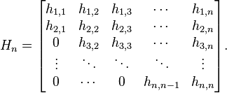
Let Q_n denote the m-by-n matrix formed by the first n Arnoldi vectors q₁, q₂, …, q_n, and let H_n be the (upper Hessenberg) matrix formed by the numbers h_j,k computed by the algorithm:

$H_n = \begin{bmatrix} h_{1,1} & h_{1,2} & h_{1,3} & \cdots & h_{1,n} \\ h_{2,1} & h_{2,2} & h_{2,3} & \cdots & h_{2,n} \\ 0 & h_{3,2} & h_{3,3} & \cdots & h_{3,n} \\ \vdots & \ddots & \ddots & \ddots & \vdots \\ 0 & \cdots & 0 & h_{n,n-1} & h_{n,n} \end{bmatrix}.$

We then have

$H_n = Q_n^* A Q_n. \,$

This yields an alternative interpretation of the Arnoldi iteration as a (partial) orthogonal reduction of A to Hessenberg form. The matrix H_n can be viewed as the representation in the basis formed by the Arnoldi vectors of the orthogonal projection of A onto the Krylov subspace $\mathcal{K}_n$.

The matrix H_n can be characterized by the following optimality condition. The characteristic polynomial of H_n minimizes ||p(A)q₁||₂ among all monic polynomials of degree n. This optimality problem has a unique solution if and only if the Arnoldi iteration does not break down.

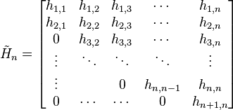
The relation between the Q matrices in subsequent iterations is given by

$A Q_n = Q_{n+1} \tilde{H}_n$

where

$\tilde{H}_n = \begin{bmatrix} h_{1,1} & h_{1,2} & h_{1,3} & \cdots & h_{1,n} \\ h_{2,1} & h_{2,2} & h_{2,3} & \cdots & h_{2,n} \\ 0 & h_{3,2} & h_{3,3} & \cdots & h_{3,n} \\ \vdots & \ddots & \ddots & \ddots & \vdots \\ \vdots & & 0 & h_{n,n-1} & h_{n,n} \\ 0 & \cdots & \cdots & 0 & h_{n+1,n} \end{bmatrix}$

is an (n+1)-by-n matrix formed by adding an extra row to H_n.

Finding eigenvalues with the Arnoldi iteration

The idea of the Arnoldi iteration as an eigenvalue algorithm is to compute the eigenvalues of the orthogonal projection of A onto the Krylov subspace. This projection is represented by H_n. The eigenvalues of H_n are called the Ritz eigenvalues. Since H_n is a Hessenberg matrix of modest size, its eigenvalues can be computed efficiently, for instance with the QR algorithm. This is an example of the Rayleigh-Ritz method.

It is often observed in practice that some of the Ritz eigenvalues converge to eigenvalues of A. Since H_n is n-by-n, it has at most n eigenvalues, and not all eigenvalues of A can be approximated. Typically, the Ritz eigenvalues converge to the extreme eigenvalues of A. This can be related to the characterization of H_n as the matrix whose characteristic polynomial minimizes ||p(A)q₁|| in the following way. A good way to get p(A) small is to choose the polynomial p such that p(x) is small whenever x is an eigenvalue of A. Hence, the zeros of p (and thus the Ritz eigenvalues) will be close to the eigenvalues of A.

However, the details are not fully understood yet. This is in contrast to the case where A is symmetric. In that situation, the Arnoldi iteration becomes the Lanczos iteration, for which the theory is more complete.

Implicitly restarted Arnoldi method (IRAM)

Due to practical storage consideration, common implementations of Arnoldi methods typically restart after some number of iterations. One major innovation in restarting was due to Lehoucq and Sorensen who proposed the Implicitly Restarted Arnoldi Method. They also implemented the algorithm in a freely available software package called ARPACK. This has spurred a number of other variations including Implicitly Restarted Lanczos method. It also influenced how other restarted methods are analyzed. Theoretical results have shown that convergence improves with an increase in the Krylov subspace dimension n. However, an a-priori value of n which would lead to optimal convergence is not known. Recently a dynamic switching strategy has been proposed which fluctuates the dimension n before each restart and thus leads to acceleration in the rate of convergence.

See also

The generalized minimal residual method (GMRES) is a method for solving Ax = b based on Arnoldi iteration.

References

• W. E. Arnoldi, "The principle of minimized iterations in the solution of the matrix eigenvalue problem," Quarterly of Applied Mathematics, volume 9, pages 17–29, 1951.
• Yousef Saad, Numerical Methods for Large Eigenvalue Problems, Manchester University Press, 1992. ISBN 0-7190-3386-1.
• Lloyd N. Trefethen and David Bau, III, Numerical Linear Algebra, Society for Industrial and Applied Mathematics, 1997. ISBN 0-89871-361-7.
• Jaschke, Leonhard: Preconditioned Arnoldi Methods for Systems of Nonlinear Equations. (2004). ISBN 2-84976-001-3
• Implementation: Matlab comes with ARPACK built-in. Both stored and implicit matrices can be analyzed through the eigs() function.